Frames of Success: Diving into the minds of movie wizards

Introduction
In this post, we try to answer to the following questions using a data-centric approach:
- Is it less or more likely for a movie to succeed when the director tries a new genre?
- Are directors who tend to work on more diverse projects less or more successful?
- To what extent do directors experiment with new genres and thematics over the course of their career?
- Are more successful directors more often specialized in a certain combination of genres?
Is it less or more likely for a movie to succeed when the director tries a new genre?
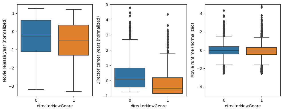
To answer this question, we can compare the success score of the movies in which the director has tried at least one new genre, with the ones in which the directors has had previous experiences with all the genres in the movie. However, simply spliting the movies into these two categories might lead to wrong inferences. There are many cofounders that could directly or indirectly impact the success of a movie. Runtime of the movie, release year, languages, production countries, genres, director, and cast could be the principal ones, among many other factors. For the purpose of this study, it is not possible to take into account all these factors, but we try to balance the dataset on the cofounders that we have data about before drawing any conclusion.
For this purpose, we match the movies exactly on the categorical features: directors of the movie, production countries of the movie, languages of the movie, and genres of the move; and calculate propensity scores for continuous features: runtime of the movie, release year of the movie, and number of years from the first appearance of the movie director in our dataset. The last feature could be a very important one because we know that even the brightest directors always need some years before finding their style. The propensity score is calculated by the coefficient of the logistic regression predictor of the probability that the director employs a new genre in the movie. The matching is then done by maximizing the sum of weights $($similarity of movies based on the difference of the propensity scores$)$ in a graph of movies with edges between movies that match exactly on the categorical features. The following figure shows the distribution of the matched variables. Although the matching is not optimal, the distributions are more or less balanced in the control and the treatment groups. Note that the normalization of the features is done before the matching, thus mean values are slightly different than zero.
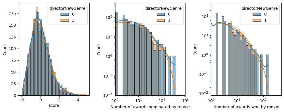
With the balanced dataset of 5250 movies, the treatment and control groups are splitted based on the exploration of a new genre by the director. We can run related t-tests on the distribution of different success metric of these two groups. The t-statistics and p-values of these tests are reported in the following table for the distribution of the movie score, the number of awards that the movie has been nominated to, and the number of awards won by the movie. For all three, the p-value is higher than 0.20 which suggests that the null-hypothesis that exploring a new genre by the director does not change the average success chances of the movie cannot be rejected.
| Metric | t-statistic | p-value |
|---|---|---|
| score | -1.2254 | 0.22 |
| awards nominated | 0.7898 | 0.43 |
| awards won | -0.6488 | 0.52 |
This can also be observed visually when comparing these distributions for both groups:
To see this further, we have fitted linear regression models for predicting the aforementioned success metrics based on the treatment feature and got the results summarized in the following table. Both the features and the metrics are standardized before fitting the linear regression models. In all cases, the coefficients are insignificant when compared to the intercepts and the corresponding p-values are larger than 0.20 which implies that we cannot reject the null hypothesis that the coefficient in this model is zero with the 20% significance level. Note that the independent variable is a categorical variable and the coefficient should be interpreted as the increase in the expected normalized score when the director tries a new genre.
| Metric | Intercept $($p-value$)$ | Coefficient $($p-value$)$ | R-squared |
|---|---|---|---|
| score | +0.0089 $($0.648$)$ | +0.0334 $($0.223$)$ | < 0.001 |
| awards nominated | -0.0571 $($< 0.01$)$ | -0.0176 $($0.427$)$ | < 0.001 |
| awards won | -0.0600 $($< 0.01$)$ | +0.0149 $($0.515$)$ | < 0.001 |
Are directors who tend to work on more diverse projects less or more successful?
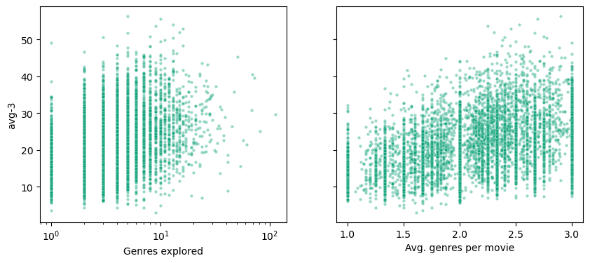
Similar to the previous question, we can compare the success score of the directors and check the correlation with a measure of tendency for more diverse projects. We do this for two measures: 1. the average number of genres per move of the director; and 2. the total number of explored genres. The dependent variable here is, the avg-3 score of the director and the number of awards of the director. The following table summarizes the results of linear regression models for predicting the dependent variable from each of the two dependent variables. Note that contrary to the previous question, here the features are not standardized. The first row shows that there is a small correlation between the average number of genres per movie and the success score. The second and the third rows show that although the positive correlations with the average number of genres per movie are insignificant with a significance level of 5%, there is a very small significant positive correlation with the total number of genres explored. The low R-squared in all the models shows that very little part of the distributions can be explained by the independent variables linearly.
| Metric | Intercept $($p-value$)$ | genresPerMovie $($p-value$)$ | genresExplored $($p-value$)$ | R-squared |
|---|---|---|---|---|
avg-3 |
+7.8017 $($< 0.01$)$ | +5.4361 $($< 0.01$)$ | 0.4017 $($< 0.01$)$ | 0.198 |
| awards nominated | +8.7994 $($< 0.01$)$ | +1.3527 $($0.057$)$ | 0.3951 $($< 0.01$)$ | 0.005 |
| awards won | +5.4011 $($< 0.01$)$ | +0.0568 $($0.865$)$ | 0.1813 $($< 0.01$)$ | 0.004 |
The figures below show the distribution of the avg-3 score versus each of the independent variables. It is evident that there is not any significant linear correlation between the score and the independent variables.
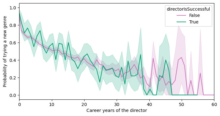
To what extent do directors experiment with new genres and thematics over the course of their career?
To answer this question, we analyze the correlation between the career years of the director in the release year of the movie with a categorical variable which indicates whether a new genre has been explored by the director in the movie. It is natural to expect a decreasing trend of trying new genres as a director goes through his career. The following table shows the results of fitting a linear regression model between these two variables considering different datasets. Note that both features are standardized before fitting the model.
| Movies | Intercept $($p-value) | directorCareerYears $($p-value$)$ | R-squared |
|---|---|---|---|
| All | +0.6804 $($< 0.01$)$ | -0.2148 $($< 0.01$)$ | 0.212 |
| Successful director | +0.6308 $($< 0.01$)$ | -0.1555 $($< 0.01$)$ | 0.159 |
| All $($after 7.5 years$)$ | +0.5380 $($< 0.01$)$ | -0.1019 $($< 0.01$)$ | 0.032 |
In the first two models, the intercept is quite high which means that with average years passed through the career of the director $($around 7.5 years$)$, the probability of trying a new genre is 0.6804 and 0.6308 among all directors and successful directors, respectively. Here, successful directors are those whose the avg-3 score is higher than 40, which includes only 135 directors in our dataset. In both models, there is a significant negative correlation between our variables. The coefficient for each row means that for each standard deviation $($around 9.3 years$)$ passed through the career of a director, the probability of trying a new genre drops as the coefficient. We notice a smaller drop among the successful directors. The third row takes into account the fact that in the first years of their career, it is naturally more probable for directors to try new genres, and takes into account only movies after at least 7.5 years through their careers. Here, again, the negative correlation exists although it is a bit milder than the other two. These negative correlations are obvious in the followin figure. Here, the mean value of binary dependent variable is plotted agains the independent variable, with 95% confidence intervals.
Are more successful directors more often specialized in a certain combination of genres?
To answer this question, we need to study not only the existence of single genres in the movies of directors, but also the co-existenec of one or more genres in their movies. Take, for instance, three comedy-romance movies, one romance-drama movie, and three drama-crime movies in a portfolio. The presense of romance genre is the same as drama $(4)$, and close to the presence of comedy $(3)$ and crime $(3)$, but these numbers alone do not represent the style of this portfolio. What is significant here, is the co-existence of comedy-romance and drama-crime movies.
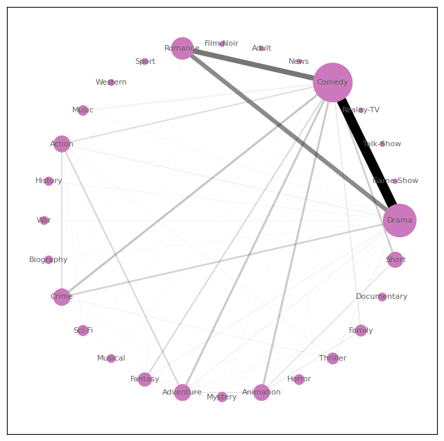
Genre co-existence graph
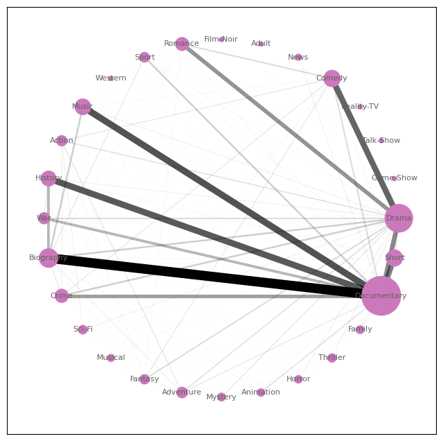
In order to get the co-existence of genres, we define a undirected bipartite graph of the movies and their genres, and draw an edge between each movie and its genres. Projection of this bipartite graph on the movies will give us a multigraph of co-existence of genres in a group of movies. The multiplicity of each edge can then be reduced to a weight to get an ordinary undirected weight graph of the co-existence of genres in a group of movies. The following graphs are visualized in the plot below. You can select a country or a decade to see the corresponding graph of the selected item. We will use the same technique to visualize the style of selected directors in the rest of this section.
Notice the transition from Short-Comedy-Drama movies in the 1900s through Comedy-Drama-Romances in the 1930s, to more emphasis on Drama and combinations with Action and Crime genres in the 2000s and 2010s. The co-existence of Drama, Action, and Romance in Indian movies is also noticable.
Genre-similarity measure
In order to get a similarity score based on the co-existence of genres, we start from the bipartite graph of a group of movies and their corresponding genres, similar to the previous section. This time, we project the plot on the genres to get a multigraph of movies. Each edge between two movies means that they have one genre in common. The maximum number of possible edges between two movies is the minimum of their number of genres. Therefore, here we reduce the multigraph to an ordinary complete weighted graph where the weight between movie $i$ and movie $j$ is defined as
\[w_{(i,j)} = \frac{\# \{\text{Common genres}\}}{\# \{\text{Maximum common genres}\}} < 1.\]In order to get an overal similarity measure for the whole graph $($all movies present$)$, we calculate the density of the weighted graph. Since the graph is complete and $0 < w_{(i,j)} < 1$, this is equivalent to summing up the weights and dividing them by the maximum possible sum of weights:
\[\text{Similarity}_{G} = \frac{2 \sum_{(i, j)} w_{(i, j)}}{N(N-1)},\]where $N$ is the number of nodes in graph $G$.
In order to have baselines for this abstract similarity score, we sample the whole movies dataset and get 100, 500, and 1000 random movies, and calculate their similarity score. We repeat this process 5 times and take the average score to get the values 0.3122, 0.3229, and 0.3059 respectively. This means that a score of around 0.30 should be considered randomly-similar. In order to have a sense of an upper bound for similarity, we calculate this score for movies from a random director with at least 10 movies and repeat this process 100 times. The average similarity score is 0.5449 this time. It means that a similarity score more than 0.50 should be cosnidered a high genre-similarity.
We now calculate the similarity of movies of top directors to get the following results:
| Description | Directors | Movies | Score |
|---|---|---|---|
| Directors with avg-3 more than 40 | 135 | 2324 | 0.33 |
| Directors with avg-3 more than 50 | 10 | 191 | 0.28 |
| Directors with avg-10 more than 40 | 18 | 418 | 0.27 |
| Directors with at least 10 movies rated 8.0 or above | 7 | 432 | 0.39 |
| Directors with at least 3 movies rated 8.5 or above | 14 | 269 | 0.40 |
| Directors with at least 150 nominated awards | 66 | 646 | 0.42 |
| Directors with at least 50 awards won | 181 | 1785 | 0.44 |
The first three rows are more or less the same as the score resulted from drawing random movies. The rest, however, show that there is actually a similarity regarding the style of the directors who have multiple highly-rated movies or have won many awards. Note that here, we filter the directors based on their characteristics and then consider all their movies, which represent their true style.
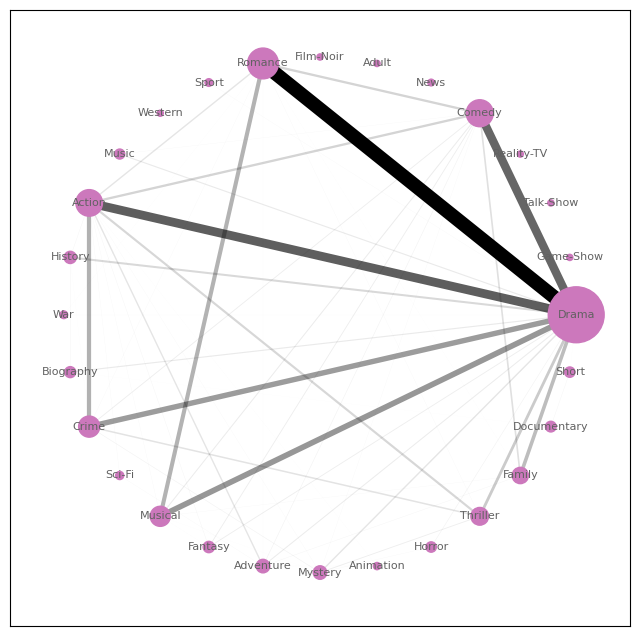
The first style comprises of Comedy, Animation and Family movies with an emphasis on the co-existence of Comedy-Animation.
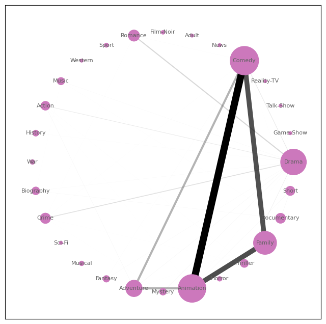
Style of 7 directors with at least 10 movies rated 8.0 or above
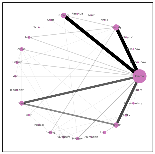
The second style comprises of Drama movies combined with Comedy, Crime, Action and Romance.
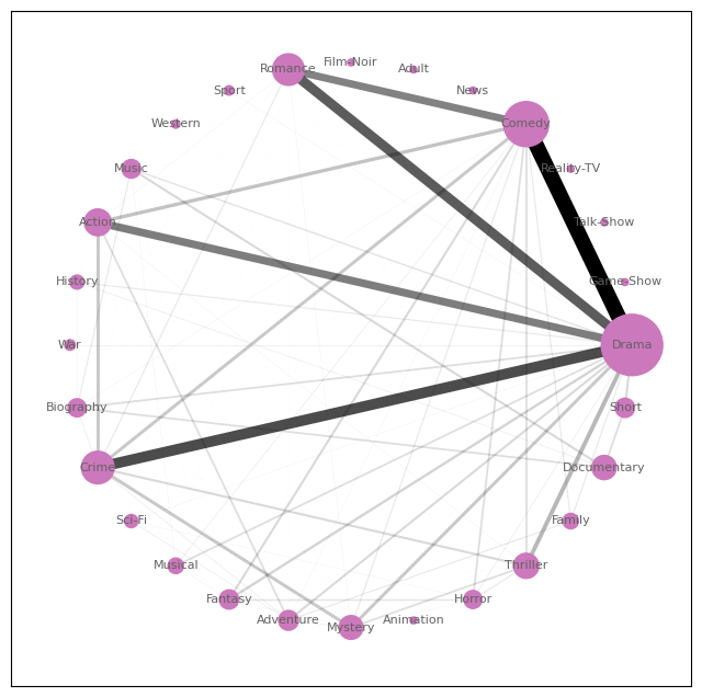
Style of 14 directors with at least 3 movies rated 8.5 or above
The third style is very similar the the second one, except that there’s less emphasis on Action movies.
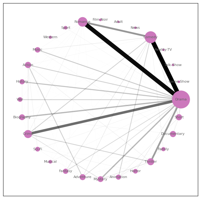
Style of 181 directors with at least 50 awards won
Next, we do the same analysis but only considering movies produced in certain countries. The results are summarized in the table below. This time, the scores are usually high, which represents the closeness in the styles of movies from the same country. The highest genre-similarity scores in the table belong to Turkey, India, and Korea. The genre co-existence graphs of these movies are presented below.
| Description | Country | Directors | Movies | Score |
|---|---|---|---|---|
| Directors with at least 10 awards won | India | 2185 | 555 | 0.61 |
| Directors with at least 50 awards won | Canada | 2185 | 429 | 0.35 |
| Directors with at least 10 awards won | Turkey | 4299 | 104 | 0.74 |
| Directors with at least 50 awards won | France | 174 | 308 | 0.54 |
| Directors with at least 10 awards won | China | 4299 | 300 | 0.57 |
| Directors with at least 10 awards won | Korea | 2185 | 163 | 0.61 |
Style of 555 Indian movies from directors with at least 10 awards
Style of 104 Turkish movies from directors with at least 10 awards
Genre-similarity measure for directors
In this part, we use a technique to draw a genre-similarity measure between each two directors among a group of directors. To do so, we create the similarity graph of the movies of the whole group as in the previous section. Next, for each pair of directors, we define the similarity between their styles as the density of the edges between their movies:
\[\text{Similarity}_{(d_1, d_2)} = \frac{\sum_{i \in d_1, j \in d_2} \text{Similarity}_{(i, j)}}{\#{d_1} \times \#{d_2}},\]where $d_1$ and $d_2$ are the set of movies from two directors. This process can be done for all the directors in the group by a reduce-based algorithm.
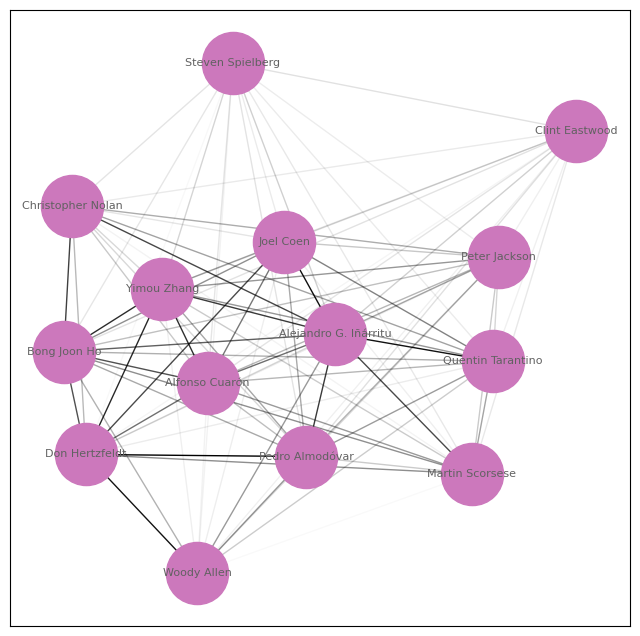
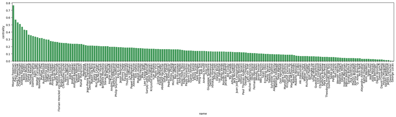
Applying this technique on the group of directors with at least 120 awards results in the following graph.
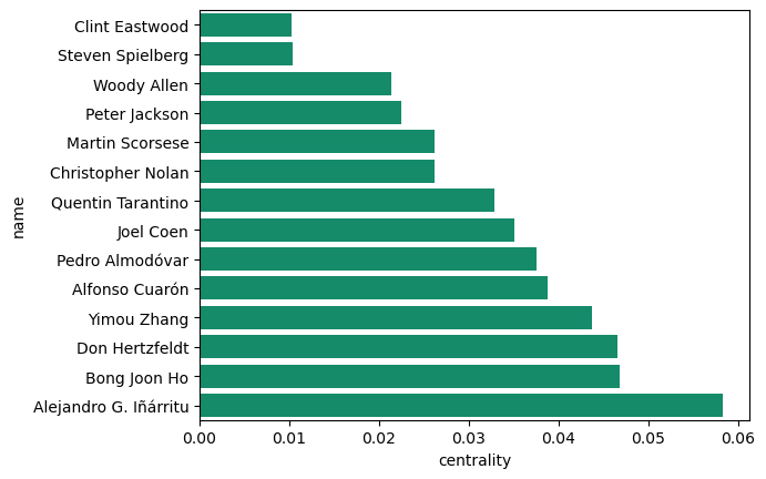
To measure how similar their work is compared to the other members of the group, we can sum the weights up and divide it by the number of other members. Doing this, we get the numbers in the figure below. We can see that directors like Clint Eastwood and Steven Spielberg, and Woody Allen have the most unique styles among the top directors of all time.
We repeat the same technique to get the ranked directors in terms of the uniqueness of their styles among the directors with at least 50 awards. The results are illustrated in the following figure. Among these directors, the ones with the most unique styles are: George Lucas, David Fincher, James Cameron, and Steven Spielberg. The ones with the most similar styles to the others are: Gary Oldman, Greg Chwerchak, Charlie Kaufman, and Andrew Kotatko.
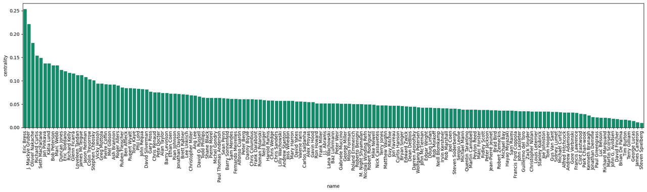
The following figure shows the same graph for directors who have at least one movie with more than 500 thousand votes on IMDb. Here we expect more similar styles because we target popular movies. We see the same names for the most unique styles as in the previous plot, and the most similar styles to the others belong to Eric Bress, J. Mackye Gruber, Olivier Nakache, and Seth MacFarlane.
Style clusters among successful directors
From the technique in the previous part, we can get a fully-connected weighted similarity graph among a group of directors. In this part, we use the adjacency matrix of such a graph and cluster the nodes $($directors$)$ using the Louvain clustering algorithm. We consider 900 directors with more than 20 awards won and analyze 6353 movies portrayed by them. Doing so, we are able to extract three major clusters.
Cluster #1
This cluster is comprised of movies in Drama, Comedy, Romance, and Crime genres and is relied on the co-existence of Drama-Romance, Drama-Crime, and Drama-Comedy. Some familiar names in this group are Joel Coen, Peter Jackson, Yimou Zhang, Martin Scorsese, and Steven Spielberg, and Christopher Nolan.

Cluster #2
This cluster is comprised of Drama, Documentary, and Short movies and is relied on the co-existence of Documentary-Biography movies, along with Crime, Histoy, and Music flavors. Directors who examplify this cluster are Lupita Nyong’o, Joe Berlinger, Bill Cosby, and James Cameron.
Cluster #3
This cluster relies on the co-existence of Comedy-Drama-Romance with an emphesis on the Comedy genre. Some familiar names in this genre are Quentin Tarantino, Don Hertzfeldt, Pedro Almodóvar, and Woody Allen.