Dive into the captivating world of cinema with our unique exploration of the CMU Movie Summary Corpus dataset. Tired of defending your love for the unparalleled duo of Ben Affleck and Matt Damon during your movie nights? You’re in the right place! Our mission, should we decide to accept it (we do), takes you on a journey where we dissect connections between actors. Discover how these links influence financial success and film quality, while exploring aspects such as geography, timeline and film genre. Thus, no more sterile debates about actor ensembles and dive into the data for an in-depth understanding of the seventh art. Get ready for an unprecedented cinematic adventure where the facts speak for themselves!
Money Talks, But Let’s Keep It Real
When we talk box office hits, we gotta make sure we’re not comparing the ’20s silent movies to today’s 3D extravaganzas without some adjustments. Money’s worth more or less depending on when you’re spending it. That’s why we adjust the cash flow from back in the day to match today’s dollars. It’s like giving old movies a fair fight in today’s box office arena.
Look at this chart right here. Once we adjust for inflation, the old correlation between a movie’s release year and its wallet—both what it cost and what it made—kinda fades away. But here’s a kicker: the relationship between what a film spends and earns? Still cozy. The more a movie’s budget balloons, the more it seems to rake in. Looks like spending big could mean earning big, but let’s not forget—correlation isn’t causation. So, let’s not jump to conclusions just yet !
Get ready to dive into the depths of data analysis and make sure you stay focused until the end of our story.
In the plot above we clearly see that the adjusted revenues are less impacted by inflation than the non adjusted ones. To proceed for this adjustement, we divided the revenues (and the budget as well) by the CPI (Consumer Price Index) taking the year 2010 as a reference. It means that we increase revenues before 2010 and reduce those after.
In this second plot, we also observe that the plot is a little more flat when we make our adjustment.
Causality between Revenue and Number of Actors
Research Objective:
In our research, we set out to investigate the relationship between the number of actors in a movie and its (log) revenue. Our initial causal diagram suggests a straightforward link, but we recognize the potential influence of confounding variables like budget, country, language and more.
Indeed, it seems like we must have the following straightforward causality :
However, numerous other variables could potentially confound causality, such as budget. Consequently, we could have a diagram that considers budget as a confounder:
Consequently, we intend to analyze this effect conditionally with respect to the primary factors,including country,language and budget magnitude. In order to exclude the effect of a possible confounder, we try to look at a subgroup of movies that share the same country,language and budget magnitude. We do not exactly proceed with a matching because the number of movies for some countries is very low but we still try to find an effect of the number of known actors on the revenues within this subgroup.
To mitigate combinatorial explosion, we opt for the group that maximizes the number of observations. The chosen features include:
- Country of Production: United States.
- Language: English.
- Budget: Magnitude equal to 108, corresponding to revenues between 107 and 108.
We exclude taking into account the year of publication due to the implementation of inflation, which already limits the impact of this variable. By extension, these actors are those playing a significant role in the film. We started with a visual exploration using boxplots :
We discern a nuanced yet positive correlation between log revenue and the number of actors, albeit not prominently evident. To comprehensively assess this relationship, we will conduct a deeper quantitative evaluation using statistical tests.
Method : Linear Regression
The initial quantitative study involved performing a linear regression, examining the relationship between the number of actors with significant roles in a film and the corresponding adjusted revenue.
Initially, the entire set of independent variables displayed significance in predicting the adjusted log-revenue (P(F-statistic) < 0.05). However, challenges emerged, such as low observations for some dummy variables. While the overall model was significant, none of the independent variables exhibited a significant impact (p-values > 0.05), indicating a high level of correlation among the variables.
To address these challenges and avoid drawing conclusions from an inconsistent model, our plan is to group the independent variables to reduce correlation. We aggregate the independent variables into groups of 5 actors (categories are now 0:0-4 actors; 1:5-9,etc.), we obtain the following beta parameters :
The revised model maintained statistical significance and a majority of the independent variables demonstrated a notable impact on log-revenue. Hence, we still discern an impact of the actor count on log-revenue within a movie group sharing the same language, country of production and budget magnitude.
We conclude that within the selected movie group sharing the same language, country and budget magnitude, we observe a meaningful impact of actor count on log revenue. However, it is essential to note that these findings may not be universally applicable to other groups due to the inability to establish clean matches.
Prediction of the revenue in function of a set of variables
The objective of this section is to construct models enabling us to forecast movie revenue by considering dependent variables such as the number of actors, the movie genre, the country of production and other relevant factors. Within our dataset, numerous categorical and numerical variables capture our interest. Consequently, we generate dummy variables for each categorical variable.
Method 1 : Monte Carlo iterations with Linear regression
Now, we have the following method that consists of applying a 1000 iterations. In each of them, we divide our dataset in train/test set.That is a fundamental step for model evaluation. We perform an OLS regression with the train set. Then, we calculate the out-of-sample (with the test set) R2. This metric gauges how well our model generalizes to unseen data. After each iteration, we meticulously document the out-of-sample R2, allowing us to construct a distribution. This distribution gives a great picture of the model’s performance variability. Below is our resulting plot :
The distribution of R2 values provides us with valuable insights into the stability and reliability of our forecasting models. We can see from the plot above that the average R2 is 0.22.
Method 2 : Iterations using Random Forest
After having plotted the distribution of R2 obtained by doing linear regressions, we try to assess the performance of the model by using random forests and also looking at the distribution of the R2. We begin by conducting a training using the function GridSearch CV(K=5). This function is used to optimize the hyperparameters of our RandomForest model. We also iterate 1000 times this method and we split the set in train/test set at each iteration. We perform a Random Forest with the train set. Then, we calculate the out-of-sample (with the test set) R2. We compute after that the distribution of the R2 within all the iterations of the Random Forests :
Initially, the random forest exhibits a commendable average predictive power (R2(rf)=0.42) with minimal variability, as indicated by a narrow confidence interval at 95% [0.38, 0.45]. Furthermore, the Random Forest demonstrates a substantial enhancement in prediction compared to linear regression (R2(lr)=0.218).
Mean Decrease in Impurity
Our objective, now, is to pinpoint the most discriminative variables within the Random Forest analysis.
In a decision tree and subsequently in a random forest, the initial selection of variables involves choosing the most informative ones to partition the dataset. The impurity, often measured by Gini impurity, defines the likelihood of a variable being selected. Therefore, a high probability indicates that the corresponding variable possesses significant explanatory power. Hence, we will visualize the dependent variables characterized by the highest Gini impurity. We plot the most important features using Mean Decrease in Impurity (MDI). The higher the MDI, the better the feature is at making predictions :
We can see that the most important features are the following : The Adjusted Budget, the Number of actors and the years. It seems quite logical that the Budget is an important predictor of the revenue. The number of actors is also an important feature and we can explain it by the fact that more complex storylines that involves a numerous set of characters and thus of actors, captivates people more. Hence, it generates more revenue. Finally, we can also hypothetically argue that the release date is also an important factor that explains revenues because people tend to spend more money on cinema than before.
Correlation between the most important features
Here is a heatmap reprensenting the correlation between each of the most important variables obtained previously from MDI :
We can see two notable information from this :
- There is a high positive correlation between English speaking movies and movies released in the USA (correlation = 0.556) which seems pretty logical.
- There is a high negative correlation between Indie movies (independent movies) and the adjusted budget (correlation = -0.2) which is also predictable since independent movies tend to have a lower budget.
Discussion about Adjusted Budget as influtential variable
Primarily, the decision trees within the random forest consistently identify the budget of a movie adjusted for inflation as the most influential dependent variable with a Gini impurity of 0.238.
The rationale is straightforward. A greater movie budget tends to yield superior outcomes in terms of special effects, set design and the caliber of hired actors that consequently leads to a higher revenue. As depicted in the graph below, this positive correlation is readily apparent, showcasing a relatively modest data spread compared to a linear model.
Discussion about other influential variables
In a previous chapter of our data exploration saga, we unearthed a positive correlation between the number of actors and adjusted revenue. The symbiotic dance unfolded—more actors, more revenue.
Our spotlight now turns to the ‘Indie’ variable, indicating whether a film is independently produced. Our previous hypothesis from the observation of the heatmap finds validation. Indeed, the variable demonstrates a negative correlation with both adjusted revenue and budget. This correlation is in line with expectations, given that independent films often face constraints in securing substantial financial backing. We can see it quite clearly in the histogram plot below where the adjusted budget for independent movies tends to be considerably lower. As a result, the earlier observed reduction in budget typically coincides with a decrease in adjusted revenue.
Delving deeper, the impact of independence resonates more profoundly in the realm of adjusted budget (rho=-0.204) compared to adjusted revenue (rho=-0.119). This observation brings a glimmer of hope to small cinema producers, suggesting that the reduction in budget doesn’t necessarily translate to a proportional decrease in revenue.
The intricate relationship between independence, budget and revenue unveils a narrative where financial constraints do not entirely dictate the destiny of independent films.
The plot clearly demonstrates what was previously mentionned since most of the observations of independent movies have an adjusted budget that is quite lower than the non-independent ones.
Industrialization of the cinema and monopole of the USA
The significance and positive correlation of the variables “Dummy_Language_English” and “Country_USA” with adjusted revenue underscore the dominance of Hollywood in the global cinema landscape from an economic standpoint. This suggests that, economically, Hollywood productions and English-language content play a pivotal role in maximizing revenue. Therefore, emphasizing the use of the English language appears to be crucial for revenue growth in the cinematic industry. Moreover, movies produced in Hollywood leverage a robust distribution network, global communication channels, marketing strategies and various other factors that contribute to revenue enhancement.
In this analysis, we note a slightly negative correlation between the production year and adjusted revenue, which is surprising. We initially expected that accounting for inflation would mitigate the impact of the production year on adjusted revenue.
Contrary to our expectations, there seems to be another variable influencing both adjusted revenue and the production year. Further exploration of this topic could unveil a potential confounding variable, adding depth to our understanding of the relationship between adjusted revenue and the year of production. However, considering that the absolute value is close to 0, it is possible that this observation is merely due to statistical noise.
A New Measure of Stardom
In the context of our cinematic project, we aim to assess the significance of interactions among various actors. The objective is to quantify the value or impact of these interactions. To pinpoint noteworthy actor pairs, we adopted the following approach:
Crafting the Lens: Our Method for Identifying Renowned Actors
Step 1: Setting the Stage with Experience
Let’s take a step back from our analysis and take a break from all the technical details to investigate the interactions between actors. We start by considering actors who have been in at least 10 movies. Why? This threshold ensures that we’re looking at actors with a substantial body of work, indicating both experience and sustained relevance in the industry. It’s not just about having a moment in the spotlight, it’s about consistent participation in the cinematic world.
Step 2: Filtration of Relevant Movies
Our goal is to enhance your movie night. Therefore, it is interesting to filter the films that are part of our dataframe. The criteria were as follows: The movie must have been translated or created in English. It must have been released after 1980. Thus, we now have a list of actors who have a role in one of the preselected films.
Step 3: Mapping the Connections
Next, we delve into the heart of our analysis - the interactions between actors. By mapping out how often actors work together, we’re able to see who’s really at the center of the industry’s collaborative network. This isn’t just about appearing on screen, it’s about being a part of the creative partnerships that defines cinema. We set a threshold for the number of interactions to focus on actors who are not only experienced but also integral to the network. Those below the threshold might have a presence, but they don’t yet form crucial links in the industry’s collaborative web. Therefore, we decide to continue with pairs of actor that played in more than 5 movies together.
The Final Curation:
The endgame of our selection process yields a curated list of actors whose interactions bear the hallmark of significance. With the final filter applied, we eliminate any film devoid of our shortlisted actors’ presence, sharpening the focus of our database. Now primed for the grand reveal, we stand on the brink of uncovering the enigmatic duo of actors that hold the keys to cinematic success.
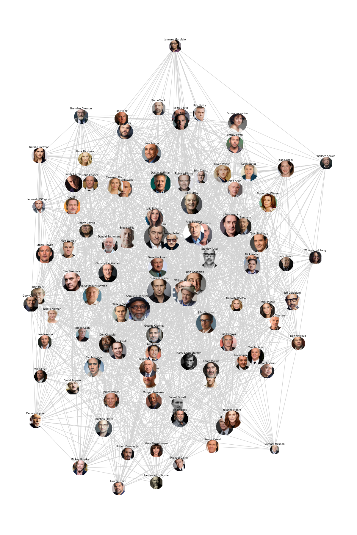
The depicted graph represents a network comprising 69 actors, providing a means to quantify the strength of interactions. Further details can be accessed by hovering over an actor’s photo. When two actors are connected, it indicates that they have collaborated in a movie. Moreover, the edges (segments connecting actor pairs) are weighted based on the total number of movies in which they have played together.
The graph’s construction offers a comprehensive understanding of how the frequency of collaborations influences actors’ positions on the cinematic stage. In constructing the graph, we employed the Fruchterman-Reingold force-directed algorithm, but to make it more accessible, let’s refer to this type of graph as a “spring graph”. In essence, envision each node as connected by a spring whose attractive force is proportional to the weight of the corresponding edge. Consequently, actors who have collaborated frequently will exhibit strong connections, tightly linked by these “springs”, while actors who have never worked together will lack any attractive forces within the graph.
Interestingly, a distinct cluster quickly emerges. Situated at the bottom right of the graph, this cluster is essentially the Harry Potter movies cluster. A significant number of actors exclusively participated in the Harry Potter film series (though they may have had roles elsewhere, our previous constraint might have filtered out lesser-known movies). As a result, all these actors are closely grouped, yet the entire cluster has shifted away from the overall mass of the graph because, in general, they did not interact with other actors. Furthermore, Harry Potter actors who also appeared in other well-known movies are positioned toward the center of the main graph due to their additional collaboration with the actors of the main cluster.
Briefly commenting on the main cluster, it is noteworthy that the distribution appears quite even. Actors of significant importance, owing to their substantial number of collaborations within our dataset, tend to occupy central positions, while those with fewer collaborations seem to gravitate toward the outer edges. Notably, actors like Steve Buscemi stand out for their astonishingly high number of collaborations compared to their peers and dominate the center.
Comparative Analysis of Revenues and Ratings
In this section, we aim to compare revenues and ratings between the filtered dataset and the remaining movies. The filtered dataset comprises movies in which at least one actor from a restricted list has played and we refer to these actors as “Renowned Actors.” This analysis aims to validate our selection process and the designation of actors in the restricted list.
Overall Analysis
In the initial analysis, we do not distinguish between datasets, comparing revenues and ratings:
| - | Renowned Actors | Non-renowned Actors |
|---|---|---|
| Mean Adj. Revenues | $127,436,562 | $58,695,708 |
| Mean Rating | 6.55 | 6.48 |
The p-value for average revenue is 1.42e-07, indicating a statistically significant difference. However, the p-value for average rating is 0.6345, suggesting no statistically significant difference.
We observe that our filtration is drastic since the difference between the bar plots of renowed actors and non-renowed actors is pretty notable. We can also see from the plot that most renowed actors tend to play in Comedy, Drama, Action, Adventure and Horror movies. And more generally we note that Drama, Comedy and Actions movies are more numerous.
Genre-specific Analysis
In the following section, we performed t-test :
Drama
| - | Renowned Actors | Non-renowned Actors |
|---|---|---|
| Mean Adj. Revenues | $63,789,276 | $40,465,501 |
| Mean Rating | 6.81 | 6.70 |
The null hypothesis is the following : H0 : The mean between the two groups is the same. We test with a 5% level. The p-value for average revenue in the Drama genre is 0.00118, indicating statistical significance. The p-value for average rating is 0.0157, also showing statistical significance.
Comedy
| - | Renowned Actors | Non-renowned Actors |
|---|---|---|
| Mean Adj. Revenues | $67,770,572 | $46,968,185 |
| Mean Rating | 6.25 | 6.19 |
The p-value for average revenue in the Comedy genre is 5.63e-7, indicating statistical significance. The p-value for average rating is 0.20, meaning the difference in average rating is not statistically significant for the Comedy genre.
Action
| - | Renowned Actors | Non-renowned Actors |
|---|---|---|
| Mean Adj. Revenues | $209,075,703 | $98,260,512 |
| Mean Rating | 6.25 | 6.21 |
The p-value for revenue is almost 0, indicating that the difference is statistically significant. The p-value for the average rating is 0.50 meaning that there is no significant difference.
Adventure
| - | Renowned Actors | Non-renowned Actors |
|---|---|---|
| Mean Adj. Revenues | $235,390,961 | $117,535,852 |
| Mean Rating | 6.51 | 6.34 |
The p-value for average revenue is 0.00016, indicating statistical significance. The p-value for average rating is 0.04 also showing statistical significance.
Horror
| - | Renowned Actors | Non-renowned Actors |
|---|---|---|
| Mean Adj. Revenues | $90,194,068 | $38,575,751 |
| Mean Rating | 6.13 | 5.67 |
The p-value for average revenue is almost 0, indicating statistical significance. The p-value for average rating is 0.016 also showing statistical significance.
Conclusion
In summary, for each genre, the difference in revenue is statistically significant, with movies featuring renowned actors earning more on average. Notably, the difference in ratings is significant for Drama, Adventure and Horror genres. Interestingly, Comedy movies, despite earning less on average, show no significant difference in ratings compared to movies with non-renowned actors.
Additionally, the comparative analysis reveals that, on average, Action movies generate significantly more revenue than Comedy movies. All these findings contribute to the robustness of our actor discrimination and the use of the term “renowned” for the restricted list.
Interaction of actors
In our quest to decipher the intricate dance of actors within the cinematic realm, we embarked on a journey armed with data on actor interactions and the films they adorned. Our primary goal was to discern the impact of actor pairings on movie revenues and ratings. With the list of actors who have a lot of interactions among themselves and the list of films in which they have played, we conduct a linear regression to identify actor pairs that have the most impact on revenues. However, we faced some problems with multicollinearity in the case that two actors play in the same exact movie. For instance, it is the case for some Harry Potter actors. We needed to take care of that so we removed actor “Duplicates”.
After dealing with this issue, we start conducting our regressions. So now, let’s refocus on the heart of our subject: the most emblematic acting duos!
Regression of the revenue on the actors and pair of actors without the budget:
We conducted a first regression in which we don’t take the budget into account. We obtained the following parameters :
We can see 3 pairs of actors that have a coefficient statistically significant. Timothy Spall & Alan Rickman, Tom Felton & Mark Williams and Jon Favreau & Vince Vaughn.
Timothy Spall & Alan Rickman, Tom Felton & Mark Wiliams are all actors of the Harry Potter saga. It’s understandable that they have opposite impact. Indeed, their interaction should compensate each other and if one of them have done another movie that is not as known as Harry Potter then it act as an outlier and undermines the revenue.
If we look at individual actor, 12 actors have a significant impact on revenue. All of them have a positive impact. It is worthy emphasizing that some of them have a slightly negative impact on revenue when they are alone and have a significant positive impact when paired with another actor, such as Jon Favreau.
We were wondering why Jon Favreau has a positive impact on the revenue while when he is paired with Vince Vaughn, suddenly the impact is significantly negative. We make the hypothesis that perhaps when these two actors play together, they usually play in comedy movies and it may be the case that comedy movies don’t generally generate high revenues. This hypothesis can in fact be supported by our previous analyzes of revenues and ratings, indeed the mean of adjusted revenues for the Comedy genre is significantly lower than the mean of adjusted revenues for the Action, Adventure and Horror genres.
Regression of the ratings on the actors and pair of actors without the budget:
We conducted a regression of the ratings on the actors and pair of actors in which we don’t take the budget into account. We obtained the following parameters :
We can see 4 pairs of actors that have a coefficient statistically significant. Ed Begley, Jr & Michael McKean, Fred Willard & Jennifer Coolidge, Eugene Levy & Jennifer Coolidge, Danny Trejo & Cheech Marin. If we look at individual actor, 20 actors have a significant impact on ratings. About half of them have a positive impact. One thing we can notice is that Fred Willard has a significant negative impact on the ratings and the pair consisting of Jennifer Coolidge and Fred Willard also have a significant negative rating, however the pair consisting of Jennifer Coolidge and Eugene Levy has a significant positive impact on the revenue.
Regression of the revenue on the actors and pair of actors with the budget:
We conducted a regression in which we take the budget into account. We obtained the following parameters :
The Adjusted budget coefficient is significant and positive which is quite predictable. This coefficient may remove the explanation linked to budget from the other previous coefficients linked to actors and pair of actors. We also encounter the same pairs as before such as Timothy Spall & Alan Rickman and Timothy Spall & Maggie Smith. If we look at individual actor, two actors have a significant impact on revenue.
Regression of the ratings on the actors and pair of actors with the budget:
Finally, we conducted a regression of the ratings on the actors and pairs of actors in which we take the budget into account:
The first thing we can mention is that the adjusted budget is not significant. We can interpret that by the fact that viewers perhaps do not necessarily care about the budget of movie to appreciate it. For the pairs of actors, they remain very similar to the previous regressions.
You can finally take a break now, no more regressions coming !
Network Analysis
Due to the limitations of the linear regression approach in quantifying the collaborative contributions of actor pairs, we found that it provided insufficient insights. The concluding sample of actors suitable for a linear regression with interactions coefficients was overly influenced by the presence of the Harry Potter cast, resulting in issues like multicollinearity. To address these challenges, we opted for a more qualitative methodology. Specifically, we pursued the construction of a revenue-based network that incorporates a larger pool of actors and adopts less arbitrary and restrictive criteria for including an actor in the dataset under current investigation.
To construct this graph, we utilized a dataset comprising over 500 available actors. Acknowledging the difficulty in effectively interpreting a graph with several hundred nodes, we opted to reduce their number based on a centrality metric. We selected the top 100 actors with the highest degree of centrality to form the foundation of our graph.
The creation of this graph employed the “spring graph” method with a focus on the top 100 actors. In a departure from our previous approach, each edge in this instance is weighted by the logarithm of the average revenue generated by movies featuring the two connected actors (as opposed to merely the count of movies they collaborated on as it was done previously). Note that the logarithmic transformation was applied for aesthetic enhancements to the graph.
We notice that after reloading the graph several times, the small clusters tend to change. So, it’s wiser not to focus too much on these details. However, the nodes consistently maintain a similar distance from the center of the graph. This suggests that, from this graph, we can recognize which actors could have easily teamed up with random actors to generate high-revenue movies by observing how close to the center they are. Nevertheless, we cannot quantitatively identify or rank the best pairs of actors by looking at this graph. Furthermore, it’s important to be aware that if two actors only did one movie together, calculating the average revenue from a single sample isn’t very meaningful. Actors with a low number of collaborations, but on high-revenue movies, will, in principle, appear closer together on the graph.
Forecasting
In the enchanting realm of cinema, the year 2024 promises a captivating array of films gracing screens around the globe. Amongst this cinematic tapestry, certain gems stand out, eagerly anticipated by audiences worldwide. If you aspire to be a cinematic trailblazer, ready to regale your friends with insights into the blockbusters set to dominate the box office, then this section is tailored just for you.
Here, we delve into the anticipation surrounding several films poised to take center stage in the cinematic landscape. Our endeavor extends beyond mere anticipation as we embark on the fascinating journey of predicting the revenues these cinematic marvels are destined to amass. Join us in this cinematic odyssey, where the magic of storytelling meets the allure of box office predictions.
Movie Releases in 2024
Madame Web
- Release Date: February 2024
- Budget: $80 million
- Number of Preponderant Actors: 8
- Genres: Crime, Drama, Thriller
Despicable Me 4
- Release Date: July 2024
- Budget: $51 million
- Number of Preponderant Actors: 2
- Genres: Kids & Family, Comedy, Adventure, Animation
Deadpool 3
- Release Date: July 2024
- Budget: Estimated $150 million
- Number of Preponderant Actors: 5
- Genres: Action, Adventure, Comedy, Fantasy
We have developed a Random Forest model and utilized it to predict the revenue of these three upcoming movies.
This is a boxplot for the three previously mentionned movies. Deadpool 3 has a median revenue of 195M $ (with q1 = 35M $ and q3 = 375M $). Despicable Me 4 has a median revenue of 54M $ (with q1 = 22M $ and q3 = 137M $). And finally, Madam Web has a median revenue of 51M $ (with q1 = 17M $ and q3 = 143M $).
Conclusion
Madame WEB
Madame Web is an upcoming American superhero film based on Marvel Comics featuring the character of the same name, produced by Columbia Pictures and Di Bonaventura Pictures in association with Marvel Entertainment. Distributed by Sony Pictures Releasing, it is intended to be the fourth film in Sony’s Spider-Man Universe (SSU).
The estimated median revenue hovers around $60,000,000, slightly below the corresponding budget. Notably, the film Morbius, belonging to Sony's Spider-Man Universe and featuring a relatively unfamiliar superhero, presents an interesting case. Despite its budget being approximately 75 million of dollars, the movie generated a revenue of 160 million of dollars. This suggests that while our predictions are reasonably close, they may benefit from factoring in the revenue boost associated with the widespread excitement surrounding Marvel movies.
In conclusion, considering these factors, we opt to forecast a gross revenue of approximately $100,000,000 for this movie.
Despicable Me 4
Despicable Me 4 is the upcoming fourth installment in the Despicable Me film series. The film’s release date is currently set for July 3, 2024.
Despicable Me 3 generated an impressive 1.035 billion in revenue, surpassing its modest budget of 80 million. The initial prediction significantly underestimated the potential revenue, projecting only 43 million. To rectify this, adjustments are necessary, considering that Despicable Me movies are animated and do not involve ‘real’ actors. Additionally, the established hype surrounding the preceding Despicable Me films should be taken into account. However, it’s essential to note that the budget for the fourth movie is reduced to 51 million, compared to 80 million for its predecessor.
In conclusion, considering these factors, we opt to forecast a gross revenue of at least $500,000,000 for this movie.
Deadpool 3
Deadpool 3 is an upcoming American superhero film based on the Marvel Comics character Deadpool, produced by Marvel Studios, Maximum Effort and 21 Laps Entertainment and distributed by Walt Disney Studios Motion Pictures. It is intended to be the 34th film in the Marvel Cinematic Universe (MCU) and a sequel to Deadpool (2016) and Deadpool 2 (2018).
The scale of your forecast for Deadpool 3 appears reasonable at 130 million, considering the success of the previous installment, which grossed 785 million with a budget of 135 million.
Given the anticipated hype surrounding this third installment, its association with the Marvel Cinematic Universe and a budget increase of 20 million, we anticipate that the revenue will likely fall within the range of 600-800 million.
Conclusion
Our journey is coming to an end, and you now possess all the necessary ingredients to become cinema connoisseurs. Initially, we tackled the issue of inflation adjustment to make our revenues comparable. We delved into causality, exploring potential confounders, but their impact proved to be less significant than anticipated. Moving forward, we ventured into predicting revenue based on various variables, uncovering several with substantial predictive power.
Next, we delved into the heart of our challenge: identifying the most iconic duos in cinema. To achieve this, we had to sift through our data to pinpoint actors with the greatest renown, employing multiple filters to select the most electrifying connections. We then conducted a comparative analysis of revenues and ratings, gaining further insights into our data. Subsequently, we examined interactions between the selected actors to deduce their most significant impact on revenue.
Finally, to wrap up our exploration, we ventured into forecasting, estimating revenue using variables with high predictive power. You now stand at the threshold of a cinematic understanding enriched by data, ready to embark on your own narrative within the vast world of film insights.
Thank you for reading our DataStory!