Full actor network characteristics
Graph generation
The actor network is modeled by a graph, where each actor represents as node \(i \in \{1 \cdots N\}\). Edges \((i,j) \in E\) are placed between two actors if they have appeared in the same movie. We additionally weigh each edge by the number of movies the two actors have in common.
Before we dive head first into computing the graph edges, we need to estimate how much space it will take. An upper bound for the number of edges is \(\mathcal{O}(\text{number of movies} \times \text{number of actors per movie}^2)\), since each movie links two actors together.
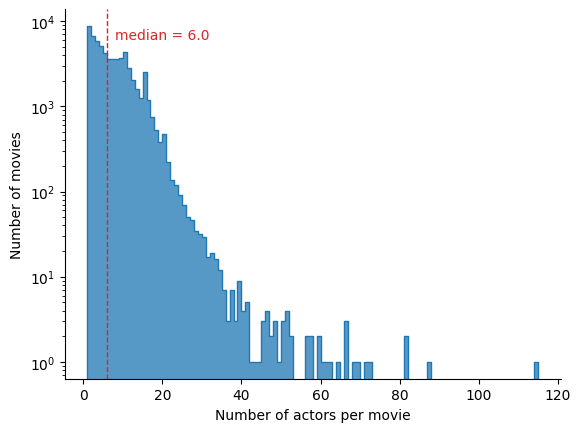
We therefore compute the number of actors per movie, and report the histogram in Figure 1.
|
numactors_per_movie |
movie_name |
| 0 |
115 |
Hemingway & Gellhorn |
| 1 |
87 |
Taking Woodstock |
| 2 |
81 |
Captain Corelli's Mandolin |
| 3 |
81 |
Terror in the Aisles |
| 4 |
72 |
Walk Hard: The Dewey Cox Story |
| ... |
... |
... |
| 64324 |
1 |
Primo |
| 64325 |
1 |
The Stranger Who Looks Like Me |
| 64326 |
1 |
On the Wing |
| 64327 |
1 |
Robot Bastard! |
| 64328 |
1 |
Incident |
64329 rows × 2 columns
With a total of 64329 movies, the distribution seems to follow an exponential law (with a somewhat long tail due to outliers). We pick the median at 6.0 to represent the distribution. We can now compute the upper bound :
With order \(10^6\) edges we will not be doing any full graph visualization, however we can do some analysis on the large graph.
After explicit computation, we get the following graph :
Graph with 135061 nodes and 2080273 edges
Thus we end up with around 2M edges (and around 2.2M edges if we keep edges between the two same actors distinct), which matches the order of magnitude estimation !
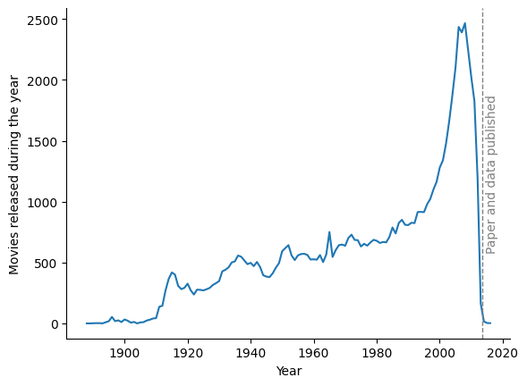
The graph contains around 135k actors, spanning movies released between 1888 and 2016, as shown in Figure 2. We note that after approximatively 2010, the number of movies in the dataset drops fast, even though the original paper with the data was published in August 2013.
Degree distribution
Among other real-life networks, social networks typically exhibit power law distribution of degrees. These types of networks are said to be “scale-free”, due to the scale-invariance of the power law. We compute the distribution for the network at hand.
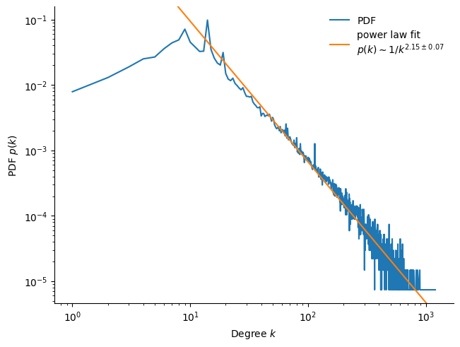
The degree distribution shown in Figure 3 clearly follows a power law \(p(k) \sim k^{-\gamma}\), and we recover the exponent \(\gamma = 1+\mu \approx 2.15 \pm 0.07\).
According to the Molly-Reed condition (Molloy and Reed 1995), the entire network is fully connected to a giant component if \(\langle k^2 \rangle < 2 \langle k \rangle\). In our case with a power law of \(\mu \approx 1.15\), the left hand side integral diverges, and so we expect to find a giant cluster. Although since \(\langle k \rangle < \infty\), we expect the giant component has not yet absorbed all clusters (“percolation”), and some smaller localized clusters remain (Bouchaud J. P. 2015).
To put this result into perspective, the Internet has in-degree distribution with \(\mu \approx 1\), scientific papers have \(\mu \approx 2\), human sexual contacts have \(\mu \approx 2.4\) (Bouchaud J. P. 2015). We are therefore in the presence of a network in which large clusters play an important role.
Clusters and diameter
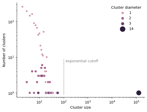
We compute the connected components of the graph (clusters), as well as their diameter. As the true diameter computation scales as \(\mathcal O(\text{number of nodes})^3\), we resort to using an approximative algorithm. Data about the 1272 clusters is plotted on Figure 4.
As expected, we indeed have a giant cluster containing \(\sim 10^5\) actors, accounting for about 94% of the total number of actors in the graph.
We also remark that even though the cluster size spans orders of magnitude, the cluster diameter spans between 1 and 14. The smaller clusters contain up to \(10^2\) actors have diameter at most 3, and their size seem to roughly follow a power law with exponential cutoff (Bouchaud J. P. 2015). Albeit its exponentially large size, the giant component has a diameter of 14, which is in-line with the small-world characteristic of scale-free networks : the diameter of the network scales only logarithmically with its size, i.e. \(d \sim \log N\) (Barabasi, Albert, and Jeong 2000).